Viscoelastic-Plastic Rheology with Transverse Isotropy¶

Fault zones in the lithosphere are thin regions of localised deformation where the mechanical response differs from the surrounding rock. They are weaker in shear along the fault plane than in the bulk, they accumulate elastic stress between slip events, and they yield when that stress exceeds a threshold. Capturing all three behaviours – anisotropic weakness, elastic memory, and plastic yield – requires a constitutive model that combines transverse isotropy (TI) with viscoelastic-plastic (VEP) rheology.

This document develops the mathematical formulation used in the TransverseIsotropicVEPFlowModel class, starting from the isotropic VEP model and the TI viscosity tensor, then showing how they combine through a resolved fault-plane yield criterion.

Isotropic Viscoelastic-Plastic Rheology¶

Maxwell Viscoelasticity¶

A Maxwell viscoelastic material partitions the total strain rate into viscous and elastic contributions:

\[ \dot\varepsilon_{ij}^{\text{total}} = \dot\varepsilon_{ij}^{\text{viscous}} + \dot\varepsilon_{ij}^{\text{elastic}} = \frac{\sigma_{ij}}{2\eta} + \frac{1}{2\mu}\frac{D\sigma_{ij}}{Dt} \]

where \(\eta\) is the shear viscosity, \(\mu\) is the shear modulus, and \(D/Dt\) denotes the Jaumann (or other objective) derivative.

Discretising the time derivative using a BDF-\(k\) scheme with leading coefficient \(c_0\) and history coefficients \(c_1, c_2, \ldots\) gives:

\[ \dot\varepsilon_{ij}^{\text{total}} = \frac{\sigma_{ij}}{2\eta} + \frac{c_0 \sigma_{ij} + c_1 \sigma_{ij}^{*} + c_2 \sigma_{ij}^{**} + \cdots}{2\mu\Delta t} \]

where \(\sigma^{*}\) and \(\sigma^{**}\) are the stress at the previous and second-previous timesteps, advected to the current particle positions (the Lagrangian stress history). Solving for the current stress:

\[ \sigma_{ij} = 2\eta_{\text{ve}}\,\dot\varepsilon_{ij}^{\text{eff}} \]

with the viscoelastic effective viscosity and effective strain rate:

\[ \eta_{\text{ve}} = \frac{\eta\,\mu\,\Delta t}{c_0\,\eta + \mu\,\Delta t}, \qquad \dot\varepsilon_{ij}^{\text{eff}} = \dot\varepsilon_{ij}^{\text{total}} - \frac{c_1 \sigma_{ij}^{*} + c_2 \sigma_{ij}^{**} + \cdots}{2\mu\,\Delta t} \]

The effective strain rate incorporates stress history: it is the strain rate that a purely viscous material with viscosity \(\eta_{\text{ve}}\) would need to produce the current stress. For BDF-1, \(c_0 = 1\) and \(c_1 = -1\); higher orders improve temporal accuracy.

The Maxwell relaxation time \(t_r = \eta / \mu\) controls the elastic-to-viscous transition. When \(\Delta t \gg t_r\), the material behaves viscously (\(\eta_{\text{ve}} \to \eta\)); when \(\Delta t \ll t_r\), it behaves elastically (\(\eta_{\text{ve}} \to \mu\Delta t / c_0\)).

Plastic Yield¶

When stress exceeds a yield threshold \(\tau_y\), the material yields plastically. In the isotropic case, yield is tested against the second invariant of the effective strain rate:

\[ \dot\varepsilon_{II} = \sqrt{\tfrac{1}{2}\dot\varepsilon_{ij}^{\text{eff}}\,\dot\varepsilon_{ij}^{\text{eff}}} \]

The effective viscosity is capped so that the resulting stress does not exceed the yield stress:

\[ \eta_{\text{vep}} = \min\!\left(\eta_{\text{ve}},\;\frac{\tau_y}{2\,\dot\varepsilon_{II}}\right) \]

This is the Drucker-Prager yield criterion expressed as a viscosity cap. The stress is then \(\sigma_{ij} = 2\eta_{\text{vep}}\,\dot\varepsilon_{ij}^{\text{eff}}\).

Transverse Isotropy¶

The Muhlhaus-Moresi Viscosity Tensor¶

A transversely isotropic material has a single weak plane defined by its unit normal \(\hat{n}\) (the “director”). The fourth-rank viscosity tensor is:

\[ \eta_{ijkl} = 2\eta_0\,I_{ijkl} - (\eta_0 - \eta_1)\left[ \frac{1}{2}\!\left(n_i n_k \delta_{jl} + n_j n_k \delta_{il} + n_i n_l \delta_{jk} + n_j n_l \delta_{ik}\right) - 2\,n_i n_j n_k n_l \right] \]

where \(I_{ijkl} = \frac{1}{2}(\delta_{ik}\delta_{jl} + \delta_{il}\delta_{jk})\) is the symmetric identity tensor, \(\eta_0\) is the bulk viscosity, and \(\eta_1\) is the viscosity for shear along the weak plane. When \(\eta_1 = \eta_0\), the anisotropic correction vanishes and the tensor reduces to the isotropic case.

The stress is:

\[ \sigma_{ij} = \eta_{ijkl}\,\dot\varepsilon_{kl} \]

The director \(\hat{n}\) typically comes from the fault surface normals, transferred to the mesh via nearest-neighbour interpolation. Far from the fault, \(\eta_1\) is set equal to \(\eta_0\) (via an influence function), so the material reverts to isotropic.

Fault Representation¶

In Underworld3, fault zones are represented as embedded surfaces. The Surface class provides:

A signed distance field from the fault
Normal vectors at each surface vertex
Influence functions that smoothly transition material properties from fault-zone values (near the surface) to background values (far away)

Available influence profiles include Gaussian (\(e^{-(d/w)^2}\)), smoothstep (\(3t^2 - 2t^3\)), linear ramp, and step function. The width parameter \(w\) controls the fault zone thickness.

A typical setup transfers fault normals to the mesh as a director field, and uses an influence function to interpolate yield stress or viscosity ratio between fault-zone and background values.

Combined TI-VEP: Resolved Fault-Plane Yield¶

The key insight in combining TI with VEP is that yield should be tested against the resolved shear stress on the fault plane, not the global stress invariant. A fault with normal \(\hat{n}\) oriented at an angle to the imposed deformation may have a low global strain rate invariant while experiencing high shear along the fault plane itself.

Viscoelastic Effective Viscosities¶

Both viscosity parameters receive the VE treatment:

\[ \eta_{0,\text{ve}} = \frac{\eta_0\,\mu\,\Delta t}{c_0\,\eta_0 + \mu\,\Delta t}, \qquad \eta_{1,\text{ve}} = \frac{\eta_1\,\mu\,\Delta t}{c_0\,\eta_1 + \mu\,\Delta t} \]

Using \(\eta_{0,\text{ve}}\) in the tensor (rather than the raw \(\eta_0\)) ensures that the anisotropic correction \(\Delta = \eta_{0,\text{ve}} - \eta_{1,\text{eff}}\) vanishes when \(\eta_1 = \eta_0\) and yield is inactive. Without this, the tensor would have a spurious anisotropic component even for isotropic materials.

Resolved Shear on the Fault Plane¶

Given the effective strain rate tensor \(\dot\varepsilon_{ij}^{\text{eff}}\) (which includes the stress history), the traction-like vector on the fault plane is:

\[ T_i = \dot\varepsilon_{ij}^{\text{eff}}\,n_j \]

This has a component normal to the fault and a component tangent to it. The normal component is:

\[ \dot\varepsilon_n = T_i\,n_i \]

The in-plane (tangential) shear magnitude follows from Pythagoras:

\[ |\dot\gamma| = \sqrt{|T|^2 - \dot\varepsilon_n^2} = \sqrt{T_i T_i - (T_j n_j)^2} \]

This formulation works in both 2D and 3D without constructing an explicit tangent vector (which is not unique in 3D). The quantity \(|\dot\gamma|\) is the magnitude of the shear strain rate resolved onto the fault plane.

Fault-Plane Yield Criterion¶

The plastic viscosity is determined by the resolved fault-plane shear:

\[ \eta_{1,\text{pl}} = \frac{\tau_y}{2\,|\dot\gamma|} \]

This is the same Drucker-Prager pattern as the isotropic case, but projected onto the fault plane. The yield-limited fault-plane viscosity is:

\[ \eta_{1,\text{eff}} = \min\!\left(\eta_{1,\text{ve}},\;\eta_{1,\text{pl}}\right) \]

In practice, a smooth approximation replaces the \(\min\) to aid solver convergence. The default “smooth” yield mode uses:

\[ \eta_{1,\text{eff}} = \eta_{1,\text{ve}}\,\frac{1 + f}{1 + f + f^2}, \quad f = \frac{\eta_{1,\text{ve}}}{\eta_{1,\text{pl}}} \]

which transitions smoothly from \(\eta_{1,\text{ve}}\) (when \(f \ll 1\), below yield) to \(\eta_{1,\text{pl}}\) (when \(f \gg 1\), above yield).

The Full Stress Formula¶

The stress is computed from the anisotropic tensor with the yield-limited viscosities:

\[ \sigma_{ij} = C_{ijkl}(\eta_{0,\text{ve}},\;\eta_{1,\text{eff}},\;\hat{n}) \;\dot\varepsilon_{kl}^{\text{eff}} \]

where \(C_{ijkl}\) is the Muhlhaus-Moresi tensor with \(\eta_0 \to \eta_{0,\text{ve}}\) and \(\eta_1 \to \eta_{1,\text{eff}}\). This naturally separates the response into:

Normal to the fault: governed by \(\eta_{0,\text{ve}}\) (pure VE, no yield)
Shear along the fault: governed by \(\eta_{1,\text{eff}}\) (VEP, yield-limited)

When the fault-plane shear stress reaches \(\tau_y\), only the fault-plane component yields. Stress normal to the fault continues to build elastically. This is physically correct: faults slip in shear, not in compression.

Using `TransverseIsotropicVEPFlowModel`¶

import underworld3 as uw
import numpy as np
import sympy

# Mesh and variables
mesh = uw.meshing.StructuredQuadBox(elementRes=(64, 64))
v = uw.discretisation.MeshVariable("U", mesh, 2, degree=2, vtype=uw.VarType.VECTOR)
p = uw.discretisation.MeshVariable("P", mesh, 1, degree=1,
                                    continuous=True, vtype=uw.VarType.SCALAR)

stokes = uw.systems.Stokes(mesh, velocityField=v, pressureField=p)

# Create TI-VEP model (order=1 for BDF-1 time integration)
cm = uw.constitutive_models.TransverseIsotropicVEPFlowModel(
    stokes.Unknowns, order=1
)
stokes.constitutive_model = cm

# Set parameters
cm.Parameters.shear_viscosity_0 = 1.0     # bulk viscosity
cm.Parameters.shear_viscosity_1 = 0.1     # fault-plane viscosity
cm.Parameters.shear_modulus = 1.0          # elastic shear modulus
cm.Parameters.yield_stress = 0.15         # fault-plane yield stress

# Director from fault normal (e.g., fault at 15 degrees from horizontal)
theta = np.radians(15)
cm.Parameters.director = sympy.Matrix([-np.sin(theta), np.cos(theta)])

The director can also be a spatially varying field (e.g., from a Surface object’s normals transferred to a mesh variable), and the yield stress can vary spatially using an influence function to localise yielding near the fault.

Smooth Yield Approximations¶

The "softmin" yield mode (default) uses a smooth approximation to \(\min(\eta_{\text{ve}}, \eta_{\text{pl}})\) to avoid the non-differentiable kink that causes problems for the SNES solver. The approximation is:

\[g(f) = 1 + \text{softplus}(f-1) - \text{softplus}(-1), \qquad \eta_{\text{eff}} = \eta_{\text{ve}} / g(f)\]

where \(\text{softplus}(x) = (x + \sqrt{x^2 + \delta^2})/2\) and \(f = \eta_{\text{ve}}/\eta_{\text{pl}}\). The offset correction ensures \(g(0) = 1\) exactly, so there is no spurious yield correction when the material is below yield.

The sharpness parameter \(\delta\) (default 0.1) controls the width of the smooth transition around the yield point. Smaller \(\delta\) gives a sharper cap (closer to the true \(\min\)) but a stiffer nonlinearity for the solver.

Choosing \(\delta\)¶

The accuracy of the smooth approximation depends on the ratio \(f_{ss} = \eta_{\text{ve}} / \eta_{\text{pl}}\) at steady state. For a simple shear problem, this simplifies to:

\[f_{ss} = \frac{\sigma_{\text{viscous}}}{\tau_y} = \frac{\eta\,\dot\gamma}{\tau_y}\]

The softmin is accurate when \(\delta \ll f_{ss}\), i.e., when the viscous stress substantially exceeds the yield stress. Practical guidance:

\(\delta\)	Accuracy at \(f_{ss} = 1.5\)	Accuracy at \(f_{ss} = 3\)	Solver cost
0.5	~85% of \(\tau_y\)	~99%	lowest
0.1	~99% of \(\tau_y\)	~100%	low
0.01	~100%	~100%	moderate

The default \(\delta = 0.1\) is accurate for all cases where the viscous stress exceeds the yield stress by at least 50% (\(f_{ss} > 1.5\)). For problems where SNES convergence is difficult at yield onset, increase \(\delta\) toward 0.3–0.5 as a relaxation parameter. Set it via cm.yield_softness = 0.1.

Benchmark Results¶

The figure below shows the TI-VEP model validated against the analytical Maxwell viscoelastic solution with plastic yield cap, for a simple shear box with an embedded fault. Two yield stresses are tested (\(\tau_y = 0.15\) and \(\tau_y = 0.30\)) at both 0 and 15 degrees fault angle. Solid curves show the analytical VE solution capped at \(\tau_y\); markers show the numerical results.

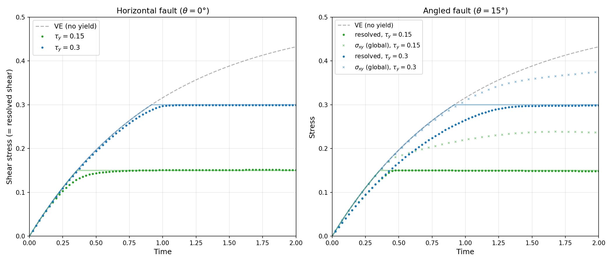
../_images/ti_vep_benchmark_final.png — TI-VEP shear box benchmark. **Left**: horizontal fault (\(\theta = 0°\)), where resolved shear equals \(\sigma_{xy}\). **Right**: angled fault (\(\theta = 15°\)), showing resolved fault-plane shear (circles) capping at \(\tau_y\) while the global \(\sigma_{xy}\) (crosses) continues to build as the bulk VE component grows. With the corrected softmin (\(\delta = 0.1\)), all cases reach within 1–2% of the analytical yield cap.¶

At 0 degrees, the resolved shear is simply \(\sigma_{xy}\) and the yield cap is exact. At 15 degrees, the anisotropic tensor creates a mechanical coupling between normal and shear components on the fault plane: the resolved shear caps at \(\tau_y\) while the global stress tensor reflects contributions from both the yielded fault-plane component (governed by \(\eta_{1,\text{eff}}\)) and the non-yielding bulk component (governed by \(\eta_{0,\text{ve}}\)).

Summary of Constitutive Models¶

Model	Viscosity	Elasticity	Yield	Anisotropy
`ViscousFlowModel`	\(\eta\)	–	–	–
`ViscoPlasticFlowModel`	\(\eta\)	–	\(\dot\varepsilon_{II}\)	–
`ViscoElasticPlasticFlowModel`	\(\eta\)	\(\mu\), BDF-\(k\)	\(\dot\varepsilon_{II}\)	–
`TransverseIsotropicFlowModel`	\(\eta_0, \eta_1, \hat{n}\)	–	–	TI tensor
`TransverseIsotropicVEPFlowModel`	\(\eta_0, \eta_1, \hat{n}\)	\(\mu\), BDF-\(k\)	\(\|\dot\gamma\|\) (fault-plane)	TI tensor

References¶

Moresi, L., Muhlhaus, H.-B., 2006. Anisotropic viscous models of large-deformation Mohr-Coulomb failure. Phil. Mag., 86, 3287-3305.
Muhlhaus, H.-B., Moresi, L., Hobbs, B., Dufour, F., 2002. Large amplitude folding in finely layered viscoelastic rock structures. Pure Appl. Geophys., 159, 2311-2333.