Tutorials
![]()
Underworld is designed to be run in the jupyter notebook environment where you can take advantage of jupyter’s rich display capabilities to explore the mathematics of your problem, visualise results and query classes or live objects.
You will find it helpful for developing scripts and analysing results. If you use jupytext to write notebooks directly as python scripts, then the same notebook codes will run on a parallel machine with no performance penalty.
The notebooks are rendered as html pages in this guide. They are distributed with the source code on GitHub and can be run on binder.
Notebook 1 - Meshes
🔗 Meshes: Introduces the mesh discretisation that we use in Underworld3 and how you can build one of the pre-defined meshes. This notebook also show you how to use the pyvista visualisation tools for Underworld3 objects. The mesh holds information on the mesh geometry, boundaries and coordinate systems.
Notebook 2 - Mesh Variables
🔗 Variables: Introduces the concept of MeshVariables in Underworld3. These are both data containers and sympy symbolic objects. We show you how to inspect a meshVariable, set the data values in the MeshVariable and visualise them.
Notebook 3 - Symbols and sympy
🔗 Symbols: meshVariables are sympy objects that can be composed with other symbolic objects and evaluated numerically when required. They can also be differentiated. Most importantly, sympy can manipulate expressions, simplify them and cancel terms.
Notebook 4 - Example: Diffusion Equation
🔗 Diffusion Solver: Introduces the various solver templates that are available in Underworld, starting with a steady-state diffusion problem. The template requires you to set some constitutive properties and define the unknowns. These are handled through subsitution into symbolic forms and the template equation can be inspected before you need to supply concrete expressions.
Notebook 5 - Poisson Equation Validation
🔗 Poisson Validation: Demonstrates how to validate the Poisson solver against known analytical solutions. We solve three progressively complex diffusion problems with linear, quadratic, and sinusoidal profiles, comparing numerical results against exact solutions.
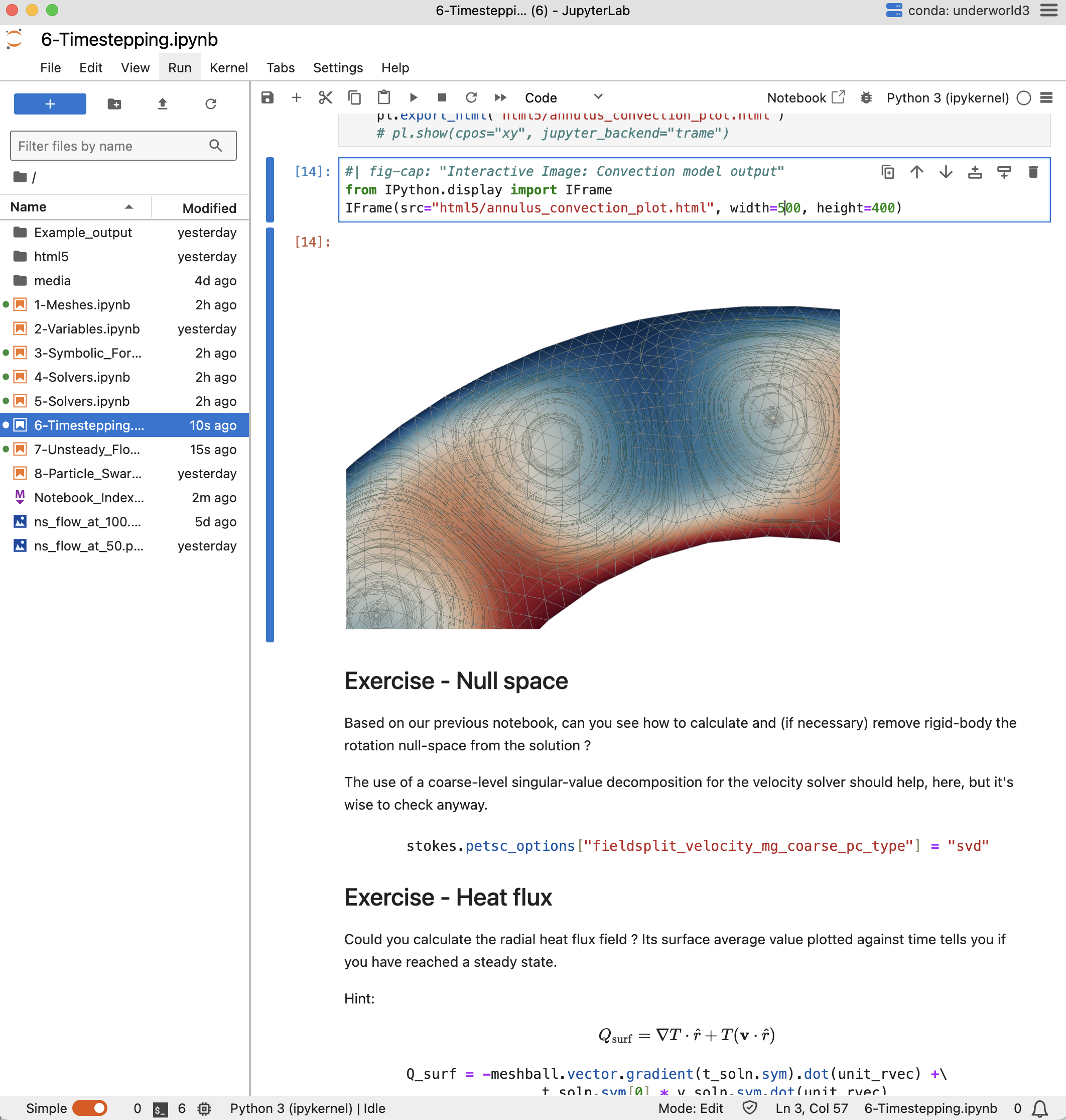
Notebook 6 - Example: Stokes Equation
🔗 Stokes Solver: Stokes equation is a more complicated system of equations to solve. This complexity is mostly hidden when you set the problem up. There are some interesting ways to constrain boundary values which are demonstrated using an annulus mesh (curved, free-slip boundaries) and a \(\delta\) function buoyancy source.
Notebook 7 - Example: Time Dependence
🔗 Timestepping: Simple advection-diffusion problem. A step (or a top-hat function) moves left to right with constant velocity and diffusion occurs at the same time. This has an analytic solution so we can see the effect of changing timesteps and grid resolution very easily.
Notebook 8 - Coupled Timestepping
🔗 Coupled Timestepping: Coupled Stokes flow plus thermal advection-diffusion gives a simple convection solver. The timestepping loop is written by hand because usually you will want to do some analysis or output some checkpoints.
Notebook 10 - Lagrangian Swarm Variables
🔗 Swarm Variables: Exploring how they work for specifying material properties with a swarm used to determine element viscosity. We learn how to use swarm variables in expressions generally and for boundary conditions.
Notebook 11 - Multi-Material Constitutive Models
🔗 Multi-Material SolCx: Demonstrates the multi-material constitutive model system by recreating the classic SolCx benchmark using IndexSwarmVariable to track different materials. Shows level-set weighted flux averaging and validation against piecewise viscosity solutions.
Notebook 12 - Working with Physical Units
🔗 Units System: Introduces physical units in Underworld3 using the Pint library. Shows how to create physical quantities (temperatures, velocities, viscosities), convert between units, work with unit-aware arrays and coordinates, and leverage automatic unit tracking through derivatives.
Notebook 13 - Non-Dimensional Scaling
🔗 Non-Dimensional Scaling: Demonstrates the non-dimensional scaling system for better numerical conditioning. Shows how to set reference quantities, solve Poisson and Stokes equations with automatic ND scaling, and validate that dimensional and non-dimensional solutions match perfectly.
Notebook 14 - Time-Dependent Advection-Diffusion
🔗 Timestepping with Units: Time-dependent advection-diffusion with physical units. Tests numerical solutions against analytical solutions for advection and diffusion of temperature steps.
Notebook 15 - Thermal Convection
🔗 Rayleigh-Bénard Convection: Complete thermal convection example with physical units. Demonstrates coupled Stokes-temperature systems with buoyancy forcing in an annulus geometry, Rayleigh number computation, and time-stepping visualization.
Notebook 16 - Richards Equation (Groundwater)
🔗 Richards Equation: Introduces the Richards equation for variably-saturated porous media flow. Solves a steady-state drainage problem in a vertical soil column using the Gardner exponential conductivity model and validates against an exact analytical solution.
Notebook 17 - Richards Equation — Transient Wetting Front
🔗 Transient Wetting Front: Solves a transient Richards equation problem where a wetting front propagates downward through a dry soil column. Validates the numerical solution against the Ogata–Banks analytical benchmark for the Gardner model.