Notebook 7: Unsteady Flow

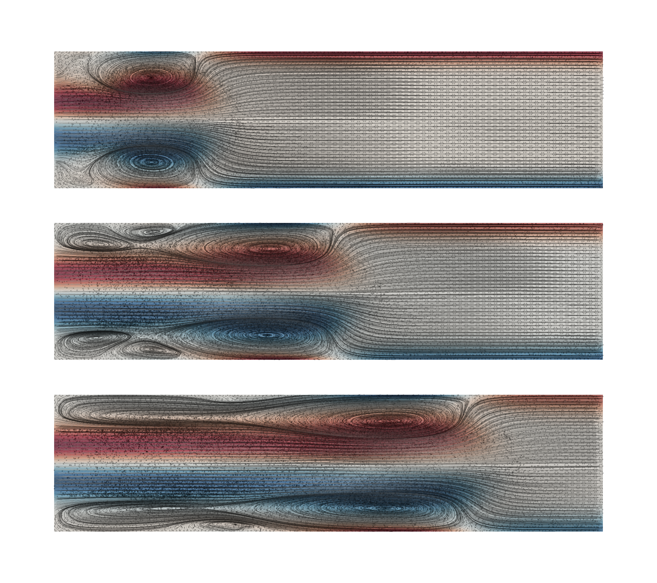
Flow in a pipe with inflow at the left boundary after 50, 100, 150 timesteps (top to bottom) showing the progression of the impulsive initial condition. For details, see the notebook code.

We’ll look at tracking an unsteady flow using a swarm of particle flow-tracers. In this case, the flow is unsteady because we solve the Navier-Stokes equation (that is, the flow has inertia) and we impose an impulsive, initial boundary velocity.

To begin with, the set up follows the same path as all previous notebooks:

• Create a mesh

• Add some variables

• Create the solver we need (NavierStokes this time)

• Add boundary conditions and constitutive properties.

We also add a projection solver to compute the vorticity of the flow as we did in Notebook 4 when we needed to compute a heat-flux (thermal gradient) term.

To track the time evolution of the flow, we introduce a “passive” particle swarm. Passive, here, refers to the fact that the flow is not changed by the presence of the marker particles.

In the time-loop we have to update the particle locations and we keep this as an explicity operation, in general, because it provide the opportunity for you to make changes or perform analyses. In this case, we are adding new particles near the inflow to track the flow.

To learn more about flow goverened by the Navier-Stokes equation, it may be he helpful to read an elementary fluid dynamics textbook and reproduce some of the simple “toy” examples. For example, Acheson, 1990.

#| echo: false  # Hide in html version

# This is required to fix pyvista
# (visualisation) crashes in interactive notebooks (including on binder)

import nest_asyncio

nest_asyncio.apply()

#| output: false # Suppress warnings in html version

import numpy as np
import sympy
import underworld3 as uw

res = 8
width = 4

reynolds_number = 1000

mesh = uw.meshing.UnstructuredSimplexBox(
    cellSize=1 / res,
    minCoords=(0.0, 0.0),
    maxCoords=(width, 1.0),
    qdegree=3,
)

# Coordinate directions etc
x, y = mesh.CoordinateSystem.X

# Mesh variables for the unknowns

v_soln = uw.discretisation.MeshVariable("V0", mesh, 2, degree=2, varsymbol=r"{v_0}")
p_soln = uw.discretisation.MeshVariable("p", mesh, 1, degree=1, continuous=True)
vorticity = uw.discretisation.MeshVariable(
    "omega", mesh, 1, degree=1, continuous=True, varsymbol=r"\omega"
)

navier_stokes = uw.systems.NavierStokes(
    mesh,
    velocityField=v_soln,
    pressureField=p_soln,
    rho=reynolds_number,
    order=1,
)

navier_stokes.constitutive_model = uw.constitutive_models.ViscousFlowModel
navier_stokes.constitutive_model.Parameters.shear_viscosity_0 = 1
navier_stokes.tolerance = 1.0e-3

navier_stokes.petsc_options["fieldsplit_velocity_mg_coarse_pc_type"] = "svd"

navier_stokes.bodyforce = sympy.Matrix((0, 0))

# Inflow boundary - incoming jet
navier_stokes.add_essential_bc(((4 * y * (1 - y)) ** 8, 0), "Left")
navier_stokes.add_essential_bc((0, 0), "Bottom")
navier_stokes.add_essential_bc((0, 0), "Top")

The Navier-Stokes Solver

The Navier-Stokes solver is a combination of a Stokes solver with time-dependent terms for both the Flux history and velocity history. These are orchestrated behind the scenes but some user-accessible options can be set, and full introspection is available using the view methods.

The velocity history terms are implemented using uw.systems.ddt objects (Eulerian, Semi-Lagrangian (default), or Lagrangian). Use navier_stokes.DFDt.view(class_documentation=True) and navier_stokes.DuDt.view(class_documentation=True) for more information.

The ddt objects implement the Adams-Moulton schemes for flux-terms (order=1 implemented the well-known Crank-Nicholson scheme). For the velocity history term, backward differentiation formulae are used. Introspection for the NS solver shows how the various terms combine to form the full set of equations.

uw.systems.NavierStokes.view()

navier_stokes.DuDt.view(class_documentation=True)

vorticity_from_v = uw.systems.Projection(mesh, vorticity)
vorticity_from_v.uw_function = mesh.vector.curl(v_soln.sym)
vorticity_from_v.smoothing = 1.0e-3
# nodal_vorticity_from_v.petsc_options.delValue("ksp_monitor")

passive_swarm = uw.swarm.Swarm(mesh=mesh)
passive_swarm.populate(
    fill_param=0,
)

# add new points at the inflow
new_points = 100
new_coords = np.array([0.0, 0.25] + 0.5 * np.random.random((new_points, 2)))
passive_swarm.add_particles_with_coordinates(new_coords)

navier_stokes.solve(timestep=0.01)
vorticity_from_v.solve()

# Keep the initialisation separate
# so we can run the loop below again without resetting
# the timer.

max_steps = 50
timestep = 0
elapsed_time = 0.0
delta_t = 0.05

for step in range(0, max_steps):

    # Keep previous guess for solve
    navier_stokes.solve(zero_init_guess=False, timestep=delta_t)
    passive_swarm.advection(v_soln.sym, delta_t, order=2, corrector=False)

    # Add new tracer particles near the inlet
    new_points = 100
    new_coords = np.array([0.0, 0.25] + 0.5 * np.random.random((new_points, 2)))
    passive_swarm.add_particles_with_coordinates(new_coords)

    # Save the data at every 10th step

    if timestep % 10 == 0:
        vorticity_from_v.solve()

        mesh.write_timestep(
            "Example_7",
            meshUpdates=True,
            meshVars=[p_soln, v_soln, vorticity],
            outputPath="Example_output",
            index=timestep,
        )

        passive_swarm.write_timestep(
            "Example_7",
            "passive_swarm",
            swarmVars=None,
            outputPath="Example_output",
            index=timestep,
            force_sequential=True,
        )

    timestep += 1
    elapsed_time += delta_t

    print(f"Timestep: {timestep}, time {elapsed_time:.4f}")

# visualise it

if uw.mpi.size == 1:
    import pyvista as pv
    import underworld3.visualisation as vis

    pvmesh = vis.mesh_to_pv_mesh(mesh)
    pvmesh.point_data["P"] = vis.scalar_fn_to_pv_points(pvmesh, p_soln.sym)
    pvmesh.point_data["Omega"] = vis.scalar_fn_to_pv_points(pvmesh, vorticity.sym)
    pvmesh.point_data["V"] = vis.vector_fn_to_pv_points(pvmesh, v_soln.sym)

    pvmesh_v = vis.meshVariable_to_pv_mesh_object(v_soln, alpha=None)
    pvmesh_v.point_data["V"] = vis.vector_fn_to_pv_points(pvmesh_v, v_soln.sym)

    skip = 1
    points = np.zeros((mesh._centroids[::skip].shape[0], 3))
    points[:, 0] = mesh._centroids[::skip, 0]
    points[:, 1] = mesh._centroids[::skip, 1]
    point_cloud = pv.PolyData(points)

    pvstream = pvmesh.streamlines_from_source(
        point_cloud,
        vectors="V",
        integration_direction="both",
        integrator_type=45,
        surface_streamlines=True,
        initial_step_length=0.01,
        max_time=1.0,
        max_steps=500,
    )

    passive_swarm_points = uw.visualisation.swarm_to_pv_cloud(passive_swarm)

    pl = pv.Plotter(window_size=(750, 750))

    pl.add_mesh(
        pvmesh,
        cmap="RdBu_r",
        edge_color="Grey",
        edge_opacity=0.33,
        scalars="Omega",
        show_edges=True,
        use_transparency=False,
        opacity=0.75,
        show_scalar_bar=False,
    )

    # Optional: plot streamlines
    pl.add_mesh(pvstream, opacity=0.3, show_scalar_bar=False, cmap="Greys_r", render_lines_as_tubes=False)

    pl.add_points(
        passive_swarm_points,
        color="Black",
        render_points_as_spheres=False,
        point_size=4,
        opacity=0.33,
    )

    # pl.add_arrows(pvmesh_v.points, pvmesh_v.point_data["V"], mag=0.1)

    # pl.camera_position = 'xy'
    pl.camera.position = (2.0, 0.5, 4)

    pl.export_html(f"html5/ns_flow_plot_{timestep}.html")

    pl.screenshot(
        f"ns_flow_at_{timestep}.png", window_size=(4000, 1000), return_img=False
    )

#| fig-cap: "Interactive Image: Time-dependent model output"
from IPython.display import IFrame

IFrame(src=f"html5/ns_flow_plot_50.html", width=1000, height=400)

Exercise - 7.1

Now that you have seen the structure of the flow in this example, can you adjust the addition of particles to capture the structure more clearly ?

This is a very low-resolution example. You can try increasing the resolution but you will see that this would benefit from running in parallel. In parallel we should remove all the visualisation and visualise the h5 output files when we are done. The rest of the code is parallel-safe.

References

Acheson, D. J. (1990). Elementary Fluid Dynamics. Oxford University PressOxford. https://doi.org/10.1093/oso/9780198596608.001.0001