Mesh adaptation by metric-driven node redistribution — mathematical formulation¶
RETIRED movers note (2026-07): the spring / Monge-Ampère / OT-step / anisotropic-Winslow interior movers this document discusses were retired (superseded by
method="mmpde", the default). Kept as the R&D record; the code lives in git history before the retirement commit.
Status: Reference (current, 2026-05) — the mathematical formulation for the implemented smooth_mesh_interior family (meshing/smoothing.py).
Scope. This is the self-contained mathematical reference for the topology-preserving mesh-adaptation family in UW3 (
uw.meshing.smooth_mesh_interior). It derives the three solution strategies — optimal-transport / Monge–Ampère, the volumetric elastic spring, and the anisotropic metric-tensor (Winslow/MMPDE) mover — the gradient-metric construction, the handling of fields under mesh motion in time-dependent problems, and the Nusselt diagnostic. Operational guidance (when to use which, parameters) is in Metric-driven mesh redistribution (smooth_mesh_interior) and Adaptive Mesh Refinement; the dated R&D log isma-newton-cofactor-exploration.md. Formulae here are transcribed fromsrc/underworld3/meshing/smoothing.py.
1. The equidistribution principle¶
All three strategies share one goal. Given a strictly-positive monitor (target density) field \(\rho(\mathbf x)\) — larger where the mesh should be finer — find a coordinate map that, at fixed topology and fixed node count, redistributes the interior nodes so the cell size tracks \(\rho\). In \(d\) dimensions the design criterion is
equivalently the equidistribution condition that the monitor mass per cell be uniform,
with \(\boldsymbol\xi\) the (uniform) computational coordinate. Boundary vertices are pinned (or slide tangentially, §6), so the domain \(\Omega\) is unchanged — this is redistribution, not re-meshing.
Important
The fixed-node-count cap. With a fixed number of nodes and fixed
connectivity, the achievable grading is bounded. For an 8–20×
density-contrast target the realisable deep/near edge-length ratio is
only ≈1.5–1.8×; the exact optimal-transport map is ≈10×. Reaching the
latter needs more nodes — a topology change (mesh.adapt / MMG), not
this smoother. Every fixed-topology local method (graph-Laplacian,
weighted-Laplacian, all Monge–Ampère variants, the elastic spring)
converges to the same ≈1.0×–1.8× band: the cap is intrinsic to
fixed-topology redistribution, not a solver deficiency. The strategies
below differ in cell shape/alignment quality and cost, not in their
ability to exceed this cap.
2. Strategy A — Optimal transport / Monge–Ampère¶
2.1 Brenier map and the Monge–Ampère equation¶
The \(L^2\)-optimal map carrying the uniform measure to the target measure \(\propto\rho\) is, by Brenier’s theorem, the gradient of a convex potential, \(\mathbf x=\nabla\Phi(\boldsymbol\xi)\). Substituting into the equidistribution condition gives the Monge–Ampère equation
Writing the map as a perturbation of the identity, \(\mathbf x=\boldsymbol\xi+\nabla\varphi\) (so \(D^2\Phi=I+D^2\varphi\)), the implementation solves
and moves nodes by \(\nabla\varphi\). The normalisation constant is chosen so that a uniform monitor is an exact no-op:
(c = 1/mean(1/sqrt(b))**2), which makes the first Picard iterate
mean-zero so that \(\rho_{\mathrm{tgt}}\!=\!\text{const}\Rightarrow
\nabla\varphi\equiv 0\).
2.2 Benamou–Froese–Oberman convex branch (2-D)¶
In 2-D, \(\det(I+D^2\varphi)=(1+\varphi_{xx})(1+\varphi_{yy})-\varphi_{xy}^2\). Setting this equal to \(g\) and solving the resulting quadratic for the Laplacian \(\Delta\varphi=\varphi_{xx}+\varphi_{yy}\) gives the two roots; the convex (Brenier) branch is the \(+\sqrt{\cdot}\) one:
(f_src = sqrt((Hxx-Hyy)**2 + 4*Hxy**2 + 4*g) - 2). The \(+\sqrt{}\)
selects the convex root unconditionally — this is what makes the
iteration stable without an explicit convexity safeguard. It is a
closed-form convex-branch solve, not a linearisation: the new
Laplacian is expressed through \(g\) and only the deviatoric part of
the Hessian, side-stepping the noisy/under-estimated full \(\det\).
2.3 Damped Picard, recovered Hessian, the move¶
The equation is solved by a damped Picard iteration: each iterate solves a constant-coefficient Poisson problem for \(\varphi\) with the above source evaluated at the previous Hessian, then under-relaxes,
without the relaxation the recovered Hessian grows unbounded and the (otherwise well-posed) Neumann solve diverges. The Poisson operator is pure-Neumann (the map’s natural BC is \(\nabla\varphi\cdot\hat n=0\)) and is closed with a constant nullspace.
Because UW3 forbids second derivatives of mesh-variable functions, the Hessian is obtained by a variationally-consistent first-derivative recovery — the SPD mass-matrix system
i.e. the weak form of \(\int H_{ij}\tau_{ij}=-\int\partial^2_{ij}\varphi\, \tau_{ij}\) integrated by parts (boundary term dropped = natural). Only first derivatives of \(\varphi\) appear.
Nodes are then displaced by \(\nabla\varphi\) subject to a coherent
global signed-area backtrack: a single scalar step factor is halved
until no triangle inverts (orientation of every cell preserved),
guaranteeing a valid mesh. (UW3’s SNES_Poisson uses \(F_0=-f\), so the
source is applied with a sign, _EQUIDIST_SIGN=-1, that makes the
validated linear first iterate \(\Delta\varphi=(g-1)\) grade nodes toward
high target density.)
2.4 The 1-D exact reference (separable features)¶
For a separable monitor (e.g. radial \(\rho(r)\) on an annulus, or angular \(\rho(\theta)\)) the exact equidistribution map is a 1-D cumulative-mass inversion, computable to machine precision with no FE solve: place node radii \(r_k\) so that equal target mass
(the \(s\,\mathrm{d}r\) is the 2-D polar area element) lies between consecutive shells, \(r_k=m^{-1}(k/N)\). This is the optimal-transport map under radial symmetry; it achieves the full ≈10× grading and is exact and strictly cheaper than any FE solve — for separable features it is the tool of choice. It also serves as the ground-truth target against which the FE strategies are measured.
Note
Why the single FE Monge–Ampère solve caps at ≈1.5–1.8×. Every FE-MA-potential variant (linear Picard; recovered-Hessian Picard, smoothed and variational; BFO convex-branch + damping; outer map composition) converges to the same ≈30 %-of-exact, self-consistent but under-deformed (non-Brenier / weak-branch) transport map — right shape and sign, never tangling, but deep/mid nodes move only ~30 % of the exact distance. This is a property of the FE-MA-potential formulation at fixed topology, not of the linear solver, Hessian recovery, branch, resolution, or single-vs-composed solves. The coupled \((\varphi,H)\) Newton SNES solves the same equation ⇒ same ceiling. Strategy C exists because a scalar potential cannot deliver coherent anisotropic bulk transport at fixed topology either.
3. Strategy B — Volumetric elastic-spring equilibrium¶
Decouple shape from size. Every mesh edge is a linear spring of uniform rest length \(\bar L\) (the current mean edge), a pure shape regulariser that drives cells equant and kills slivers; the size grading lives entirely in a per-cell area target. Minimise the truss energy
with per-cell target area \(A^0_t\propto 1/\rho_{\mathrm{tgt}}\), rescaled so \(\sum A^0_t=\sum a^{\text{init}}_t\) (total area conserved — pure redistribution). Defaults \(w_{\text{shape}}=1,\ w_{\text{size}}=8\); results are robust to them. Minimised by Jacobi-preconditioned nonlinear conjugate gradients (Polak–Ribière\(^+\)) with an Armijo line search that rejects any cell-inverting trial — the tangle guard lives inside the optimiser, so it converges to the true equilibrium rather than creeping against a per-sweep freeze. Fast (≈0.3 s on a res-16 annulus), robust, never degenerates; slightly streaky/anisotropic at sharp interior features.
4. Strategy C — Anisotropic metric-tensor mover (production)¶
A scalar equidistribution potential is isotropic and, at fixed topology, cannot produce coherent anisotropic bulk transport. Strategy C instead reshapes cells with a gradient-derived anisotropic metric tensor and an M-weighted harmonic (Winslow / MMPDE) coordinate map.
4.1 The gradient-derived metric tensor¶
From the scalar density \(\rho\), form the projected gradient
\(\nabla\rho\) (a first derivative — UW3-clean; via a
Vector_Projection), and at each node build
(M = base*(I + beta*(gn/gref)**2 * outer(gh,gh))), then
eigen-clamp: \(M=\sum_i\lambda_i\mathbf v_i\mathbf v_i^{\mathsf T}\),
clip \(\lambda_i\in[\,1/h_{\max}^2,\;1/h_{\min}^2\,]\) with
\(h_{\min}=h_0/\sqrt{\texttt{aniso\_cap}}\),
\(h_{\max}=h_0\), and reassemble. \(h_0\) is the mean edge length;
\(\nabla\rho_{\mathrm{ref}}\) the max projected \(|\nabla\rho|\).
The eigenframe auto-aligns to the feature from the Cartesian \(\nabla\rho\) alone — no \((r,\theta)\) frame is supplied anywhere (figure below). A radial feature yields tangentially-elongated cells (short \(\perp\hat{\mathbf r}\), long along the ring); an angular feature yields radially-elongated cells. Being a gradient metric it refines where \(\rho\) changes (feature edges/flanks) and is isotropic-coarse at a smooth peak (\(\nabla\rho\to0\)) and in the far field — the correct behaviour for resolving fronts/interfaces; resolving a feature core needs a curvature (Hessian) metric instead.
Single-knob equidistribution (resolution_ratio)¶
The anisotropic term is positive-semidefinite, so the bare metric is
\(M\succeq\tfrac1{h_0^2}I\): it can only refine (it keeps just
\(\nabla\rho\) and discards \(\rho\)’s magnitude, so it never asks for a
cell coarser than \(h_0\)). On a fixed node budget that is fatally
one-sided — flat regions cannot release nodes, the globally-steepest
feature scavenges the budget and the interior plumes starve. This is
structural, not a tuning deficit: no aniso_cap, \(\beta\), or
percentile setting frees the budget; they only re-aim one that is
never released.
The fix makes the isotropic part a genuinely equidistributed density. Evaluate \(\rho\) on the (near-uniform, undeformed) metric mesh, form the geometric mean \(G=\exp\langle\ln\rho\rangle\), and set
eigen-clamped to \(\lambda_i\in[\,1/h_{\max}^2,\,1/h_{\min}^2\,]\) with \(h_{\min}=h_0/R\), \(h_{\max}=h_0R\) for the single knob \(R=\texttt{resolution\_ratio}\). Because \(\langle\ln s\rangle=\ln (1/h_0^2)\), the node budget is centred: steep regions (\(\rho>G\)) refine and flat regions (\(\rho<G\)) coarsen by exactly complementary amounts — the conservation law of §1 supplies the de-resolution automatically; there is no coarsening parameter. M-harmonic scale-invariance makes the normalisation constant irrelevant to the realised mesh, so \(G\) only serves to place the clamp band symmetrically about the bulk; \(R\) alone bounds the realised fine:coarse ratio at \(R^2\). \(R=1\) collapses the band → the metric reverts bit-identically to the refine-only historical default (an exact no-op vs. every prior result); \(R\!\approx\!2\) is the validated production point.
Why a single normalised knob rather than two caps. The earlier two-knob form (\(s=h_0^{-2}\texttt{coarsen\_cap}^{\,q-1}\), separate \(h_{\min}\)/\(h_{\max}\)) exposed the refine⇄coarsen split as a free parameter, and a sweep showed that split is not free — it is a single quality budget with a sharp knee:
legacy |
\(\min A/\overline A\) |
edge p95/p05 |
mesh |
|---|---|---|---|
4 (refine-only) |
~0.27 |
~2.0 |
clean, no de-resolution |
6 (cc 1.5) |
0.20–0.25 |
~3.4 |
clean, subtle grading |
8 (cc 2) |
0.17–0.23 |
~3.8 |
clean, clearly graded |
16 (cc 4) |
0.04–0.14 |
~5.4 |
sliver mess (over-coarse) |
The good operating point was asymmetric (refine \(2\times\), coarsen
only \(\approx1.4\times\)): over-coarsening slivers the flats. The
equidistribution normalisation makes that balance automatic and
field-adaptive instead of a hand-tuned cap product — flat regions
release exactly the budget the fronts consume, so the user sets only
how much resolution range (\(R\)), never where the split lies. The
legacy aniso_cap/coarsen_cap pair is retained solely as a
bit-for-bit expert override for \(R\le1\) so historical scripts
reproduce; resolution_ratio is the documented API.
Temporal damping of the normaliser. \(G\) is recomputed from the instantaneous field at every adaptation event. The eigen-clamp band \([\,b/R^2,bR^2\,]\) is fixed, but \(G\) floats; during a violent transient (e.g. the \(\mathrm{Nu}\!\approx\!17\) convective overshoot) a \(G\) excursion translates the whole \(\rho/G\) distribution sideways across that fixed band, so a large fraction of nodes simultaneously saturate against a clamp limit and the mesh visibly lurches — and even in steady state the fine⇄coarse contrast pulses as \(G\) breathes. Because \(G\) is geometric, low-pass it in log space across events,
with \(a=\texttt{geom\_mean\_smoothing}\) (\(a\!=\!1\) ⇒ no damping / instantaneous; \(a\!\approx\!0.25\) ⇒ strongly damped; the first event seeds the state). This smooths only the single global intensity scalar — the spatial \(\rho(\mathbf x)\) pattern still tracks the current field every event, so where the mesh refines stays fully responsive; only the global de-resolution magnitude is time-filtered. It is an internal constant (one carried scalar, not a grading knob): the user-facing API stays single-knob. Equivalent to equidistributing a time-averaged density — for a slowly evolving field arguably more desirable than chasing every fluctuation, and strictly better through the startup transient.
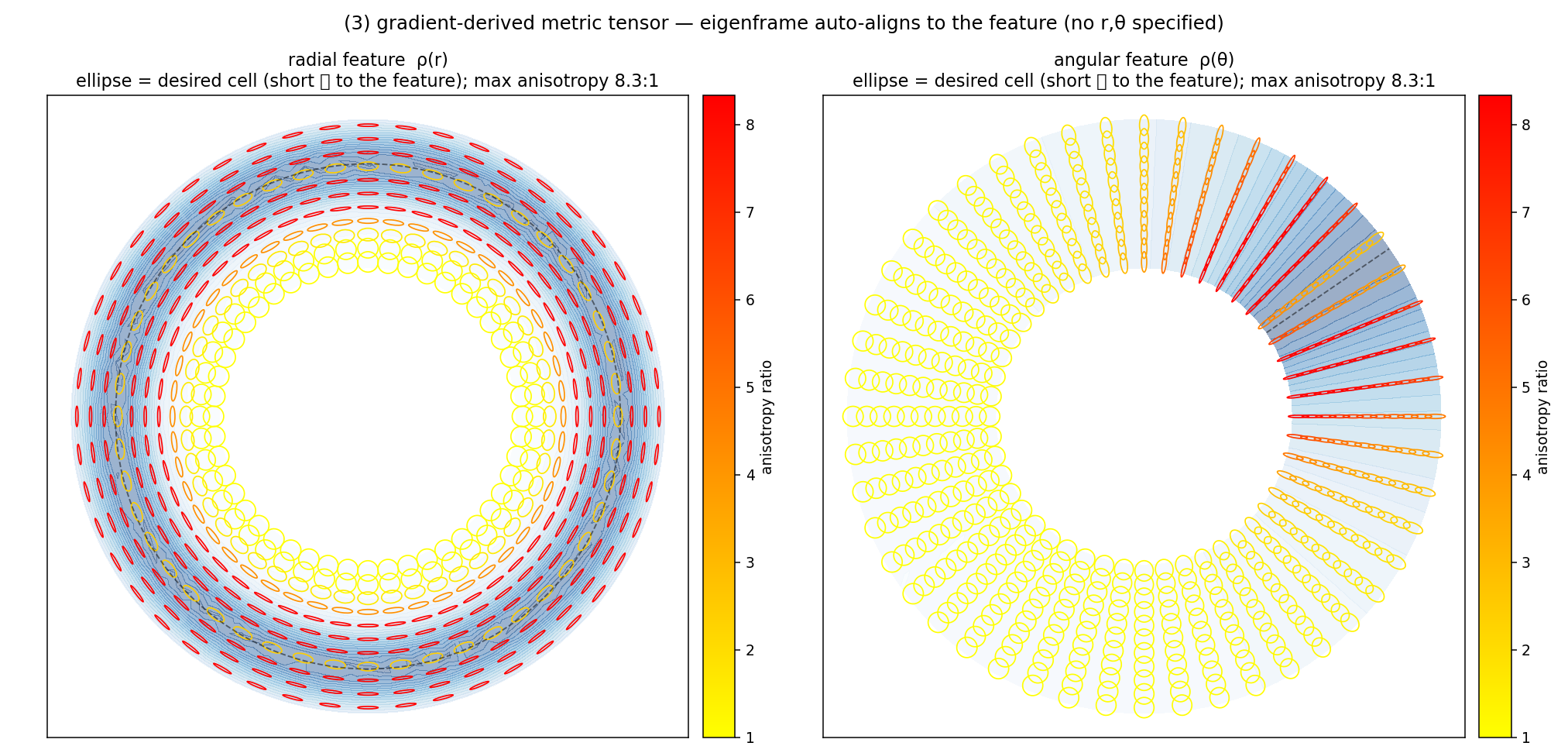
The eigen-clamped metric tensor for a radial \(\rho(r)\) (left) and an angular \(\rho(\theta)\) (right): desired-cell ellipses (short axis \(\parallel\nabla\rho\)). The eigenframe aligns to \(\hat{\mathbf r}\) / \(\hat{\boldsymbol\theta}\) purely from the Cartesian \(\nabla\rho\); the anisotropy is bounded by the eigen-clamp band.¶
4.2 The M-weighted (Winslow) coordinate map¶
Solve the displacement form of the M-weighted Laplace map, per physical coordinate component \(c\),
with \(D=M\) the eigen-clamped tensor (src = Σ_j Dsym[j,c].diff(X[j])).
Then \(\psi_c=x_c+u_c\) is exactly the M-harmonic coordinate map
\(\nabla\!\cdot(D\nabla\psi_c)=0\), \(\psi=x\) on the boundary (since
\(\nabla x_c=\mathbf e_c\)). The 1-D analysis \((D\psi')'=0\) gives
\(\psi'\propto1/D\), so the direct Winslow smoother clusters nodes
where \(D\) is large — hence \(D=M\) (large eigenvalues = small target
spacing) grades the mesh toward the metric. The two components share
the same tensor operator (a _CofDiff-style DiffusionModel with
\(\mathbf c=D\)); the system is linear (one solve per component, no
Picard) and homogeneous-Dirichlet ⇒ non-singular (no constant
nullspace, side-stepping the GAMG-pure-Neumann fragility). The overall
scale of \(D\) is irrelevant — the PDE is invariant under \(D\to\alpha
D\) — only its anisotropy and spatial variation matter; the \(1/h_0^2\)
normalisation only fixes the interpretation of the eigen-clamp band.
The displacement is applied with the same coherent signed-area backtrack as Strategy A.
4.3 Stability — damped MMPDE¶
The decoupled, direct Winslow form (each physical coordinate
M-harmonic independently) has no Rado–Kneser–Choquet non-folding
guarantee, so a single un-damped elliptic jump folds. It is therefore
run as a damped MMPDE: the metric tensor is built once on the
undeformed mesh and held fixed-Lagrangian (re-projecting \(\nabla\rho\) on
the progressively distorted mesh is a positive feedback that collapses
the mesh); the displacement is under-relaxed,
\(\mathbf x\leftarrow\mathbf x+\texttt{relax}\cdot\mathbf u\), and
composed over n_outer steps. The binding stability lever is the
eigen-clamp aniso_cap, not \(\beta\): aniso_cap≈2 is robust at
relax≈0.1–0.2; ≈4 is clean with a gentler relax≈0.05 and more
n_outer; ≳6 folds regardless (that would need the coupled/inverse
Winslow — out of scope). A scale-aware floor g_eps makes a
(near-)uniform \(\rho\) an exact identity (it rejects the
\(\sim10^{-18}\) round-off of the projected zero gradient, which would
otherwise be percentile-normalised into a spurious metric).
5. Metric construction from a field gradient¶
For the common case “refine where field \(f\) has steep gradients” the
helper uw.meshing.metric_density_from_gradient builds the relative
target density
with \(g_{\mathrm{lo}},g_{\mathrm{hi}}\) the lo/hi percentiles of the
projected \(|\nabla f|\). This is the deliberate, intent-identical
analogue of uw.adaptivity.metric_from_gradient (which maps the same
normalised \(|\nabla f|\) to an absolute target edge length
\(h\in[h_{\min},h_{\max}]\) for the MMG re-mesher). The distinction is the
node budget:
Important
amp is a no-op for the anisotropic mover (Strategy C); the
effective metric-construction knobs are the percentile window and,
in the mover, aniso_cap/\(\beta\). Strategy C builds \(M\) from
\(|\nabla\rho|/g_{\mathrm{ref}}\) with \(g_{\mathrm{ref}}=\max|\nabla\rho|\)
(§4.1). With \(\rho=1+\texttt{amp}\cdot t\) both \(|\nabla\rho|\) and
\(g_{\mathrm{ref}}\) scale linearly with amp, so it cancels
exactly — \(M\) is independent of amp (verified to machine
precision; amp=16 vs 24 give bit-identical metrics). What does
not cancel is the percentile window
\((g_{\mathrm{lo}},g_{\mathrm{hi}})\): it reshapes \(t\) (which gradient
quantile is clipped flat vs in the linear ramp), hence \(\nabla t\),
hence \(M\) — so it chooses which gradient strength triggers
refinement. For the mover the user-facing model is now a single
knob, resolution_ratio \(R\) (§4.1): it sets the resolution range
(\(h_0/R\) … \(h_0R\)) while the equidistribution normalisation supplies
the complementary coarsening automatically — there is no separate
budget/percentile/coarsen lever to balance. The percentile window
still shapes where the gradient counts as a front (a property of
metric_density_from_gradient, upstream of the mover), but the
refine⇄coarsen split is no longer a parameter. amp is inert here
but is a real bunching intensity for the isotropic spring /
Monge–Ampère methods (where the absolute \(\rho\) magnitude enters
\(A^0\propto1/\rho\) and \(g\propto1/\rho\)) — it is method-dependent.
|
|
|
|---|---|---|
mechanism |
re-mesh: insert/remove nodes |
redistribute existing nodes |
metric target |
absolute \(h\) |
relative density \(\rho\) |
variables |
reset (must transfer) |
preserved (topology fixed) |
Important
The metric is \(1/h^{2}\) per principal direction in 2-D and 3-D — not \(1/h^{d}\). A Riemannian metric measures edge length (a 1-D quantity: \(\mathbf e^{\mathsf T}M\mathbf e=1\Rightarrow\) eigenvalue \(1/h^2\)), independent of embedding dimension. Dimension enters only the element-count integral \(\int\!\sqrt{\det M}\,\) via \(\det M=\prod_i 1/h_i^2\). So the 3-D extension keeps the same construction; no exponent change.
6. Dynamic adaptation — fields under mesh motion¶
In a time-dependent problem the mesh is adapted every few steps. The
mover only moves coordinates: _deform_mesh rewrites the coordinate
vector and invalidates caches but never touches MeshVariable data,
so fields are Lagrangian-carried (DOF values unchanged, their
support relocated). Used uncorrected, this injects the pure mesh
displacement as a spurious advection. Two corrections:
Interpolation / remap (general, solver-agnostic). Because this adapter is topology-preserving (vector size, DOF order and the parallel partition are invariant) and the boundary is pinned (domain unchanged, every new node in-domain), the old field can be evaluated at the new node positions by the local FE evaluate at maximum fidelity (true P3 basis, no cross-rank migration) — distinct from, and much sharper than, the kd-tree
read_timesteppath used for the decomposition-changingmesh.adapt. This is the relative-budget analogue of the standard re-mesh-then-transfer workflow.ALE (specialised). Keep the Lagrangian carry but drive the advection–diffusion solver with the relative velocity \(V_{\mathrm{fn}}=\mathbf v-\mathbf v_{\mathrm{mesh}}\), \(\mathbf v_{\mathrm{mesh}}=\Delta\mathbf x/\Delta t\). Requires the adapter to be bound to that solver (a coupling the remap does not need); avoids interpolation diffusion.
Important
Pristine re-mesh for the dynamic loop. Re-adapting the already-graded mesh each event compounds compression (mesh quality collapses over ~tens of events). The fix — the across-events analogue of holding the metric Lagrangian within a call — is to re-derive the adapted mesh from the original node positions at every adaptation: each event is a single, fresh uniform → graded map, so compression is bounded to single-adaptation quality indefinitely. With this, the strong-metric setting stays healthy over a full saturated run.
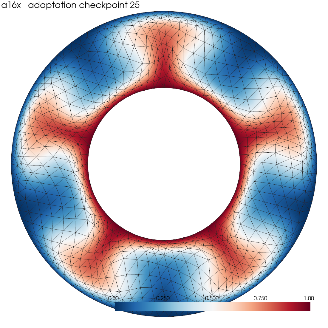
Applied example: Ra=10⁵ annulus thermal convection, res-16 base mesh,
pristine re-mesh every 5 steps with a strong \(|\nabla T|\) metric. The
mesh grades into the inner thermal boundary layer and the plume
conduits while the cells stay well-shaped. Animate with
scripts/aniso_movie.py.¶
7. Validation summary¶
Validated with anisotropy-aware diagnostics (radial/tangential
edge-length split and minA/meanA, not the anisotropy-blind d/n)
against the exact 1-D OT reference.
The anisotropic mover (C) is the cleanest method everywhere (
minA/meanA2.6–12× better than the isotropic Monge–Ampère, never slivers), linear and cheap.It does not beat the fixed-node-count cap (§1); for separable features the exact 1-D OT (§2.4) is strictly better and cheaper. It earns its keep on non-separable features and on cell alignment/quality.
In a dynamic Ra=10⁵ adaptive run the adapted res-16 mesh reproduces the res-24 reference’s heat transport (Nu within ≈1 %) and kinetic energy (\(v_{\mathrm{rms}}\) within ≈3 %) at ≈0.69× the reference wall-time; the adaptation overhead itself is a small fraction of one Stokes solve.
Single-knob equidistribution (
resolution_ratio), fully validated. Gating/clamp probe: \(R\!=\!1\) has no sub-baseeigenvalue and ratio \(=\)aniso_capexactly (the refine-only no-op, confirmed empirically as well as by construction); \(R\!=\!2\) respects the clamp \([\,b/4,4b\,]\) with 0 violations, eigenvalues spanbaseboth ways, \(\approx\)62 % of nodes coarsened to fund the fronts (parameter-free complementary de-resolution). A fresh→saturation Ra=10⁵ run at \(R\!=\!2\) (a16e, 326 steps, 65+ adaptation events) holdsminA/meanA\(\approx\)0.20 with zero folds through the full overshoot→settle cycle and settles at \(\mathrm{Nu}\approx3.87\) — quantitatively matching the hand-tuned legacy two-knob point (coarsen_cap=2:minA/meanA\(\approx\)0.20, \(\mathrm{Nu}\approx 3.89\)) with one parameter-free knob. The geometric-mean centring self-lands in the sliver-safe regime; the user sets only the resolution range, never the refine/coarsen split.
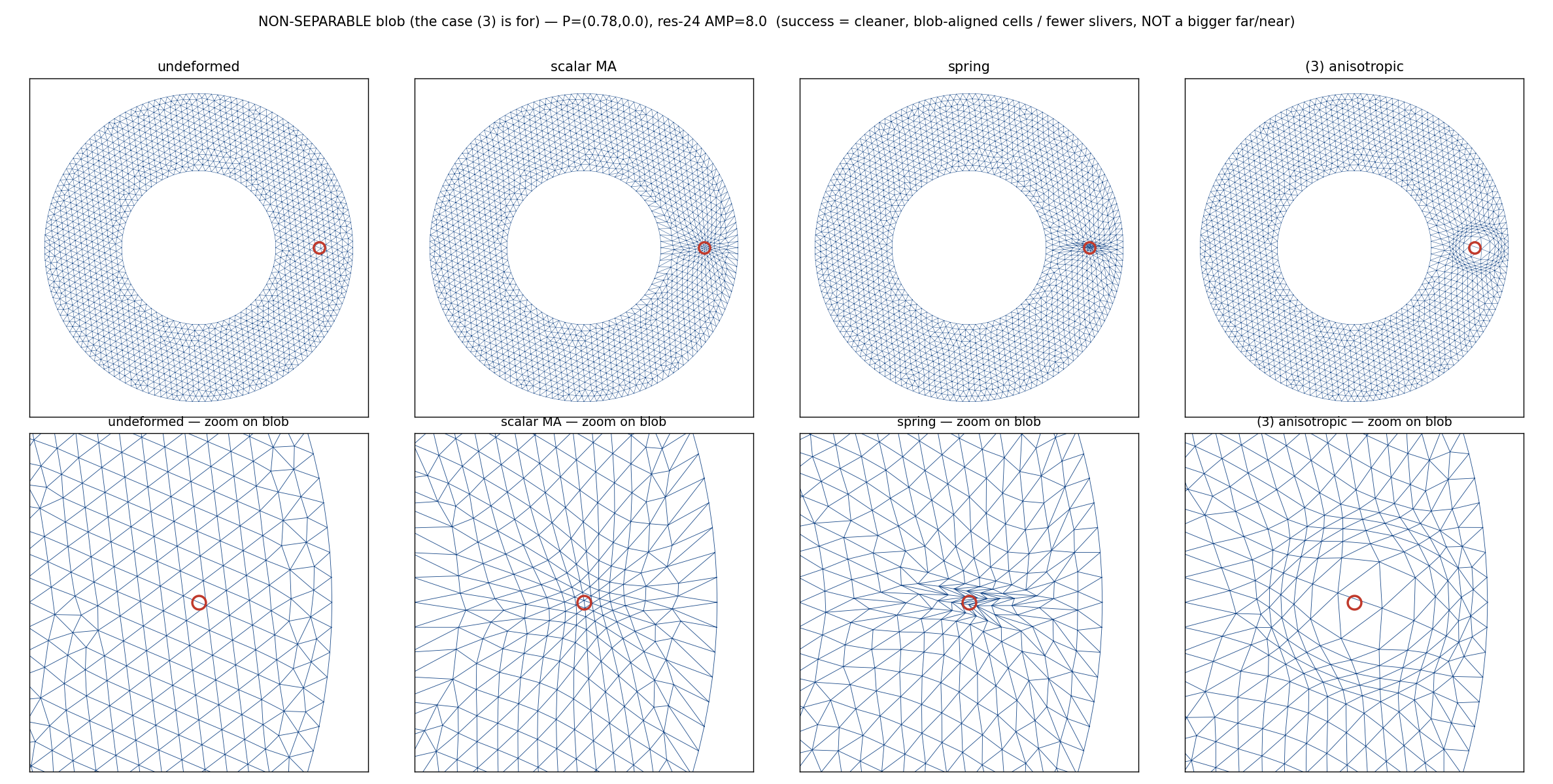
Non-separable Gaussian blob: target metric (top-right), the realised anisotropic-mover mesh, and zooms vs the isotropic Monge–Ampère / spring. The tensor mover produces clean, blob-aligned cells where the scalar methods pull a degenerate slivered knot.¶
8. The Nusselt diagnostic¶
Heat transfer is reported as the measured total radial heat flux relative to the conductive flux. The total radial flux density is \(q_r=v_r\,T-\partial_r T\) (advective + diffusive). It is projected to a nodal field and integrated over an interior shell:
At steady state \(Q(r)\) is shell-independent (conservation), and an interior shell is immune to thermal-boundary-layer resolution — unlike a near-wall \(\partial T/\partial r\) stencil, which under-resolves a sub-element boundary layer and reports ≈2–3× too low. The conductive normalisation uses the true annular conduction solution of \(\nabla^2T=0\) with \(T(R_i)=1,\,T(R_o)=0\), which is logarithmic \(T_{\mathrm{cond}}=\ln(r/R_o)/\ln(R_i/R_o)\) (not the linear slab profile used for the Boussinesq buoyancy reference), giving the total conductive flow
By construction \(\mathrm{Nu}=1\) at pure conduction (verified to \(1.0000\) on the analytic profile, shell-independent). Note the local conductive flux density is \(1/(r\ln(R_o/R_i))\approx1.4\)–\(2.9\) (Cartesian-like ≈2), while \(Q_{\mathrm{cond}}\approx9.06\) is the total power through the circumference; the Nu ratio is invariant to this choice.
References & cross-links¶
Metric-driven mesh redistribution (smooth_mesh_interior) — operational guide (parameters, when to use which).
Adaptive Mesh Refinement — user-facing, alongside
mesh.adapt.docs/developer/design/ma-newton-cofactor-exploration.md— the dated R&D log (Newton/cofactor, GAMG, the validation arc).Implementation:
src/underworld3/meshing/smoothing.py(_winslow_elliptic,_winslow_spring,_winslow_anisotropic,metric_density_from_gradient). Reproduce the figures withscripts/ma_metric_tensor_viz.py,scripts/aniso_validate_*.py,scripts/adaptive_saturation*.py,scripts/aniso_movie.py.